
Day 1: Of Numerical Integration and Python
Contents
![]()

Day 1: Of Numerical Integration and Python
Welcome to Day 1! Today, we start with our discussion of Numerical Integration.
What is Numerical Integration?
where, \(x\) is an \(N-\)dimensional vector and \(t\) typically stands for time. The function \(f(x,t)\) may be a nonlinear function of \(x\) that explicitly depends on \(t\). In addition to specifying the form of the differential equation, one must also specify the value of \(x\) at a particular time point. Say, \(x=x_{0}\) at \(t = t_0\). It is often not possible to derive a closed form solution for this equation. Therefore numerical methods to solve these equations are of great importance.
Euler’s Method for Numerical Integration
We use Euler’s Method to generate a numerical solution to an initial value problem of the form:
Firstly, we decide the interval over which we desire to find the solution, starting at the initial condition. We break this interval into small subdivisions of a fixed length \(\epsilon\). Then, using the initial condition as our starting point, we generate the rest of the solution by using the iterative formulas:
to find the coordinates of the points in our numerical solution. We end this process once we have reached the end of the desired interval.
The best way to understand how it works is from the following diagram:

Euler’s Method in Python
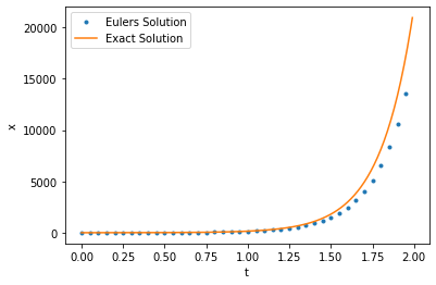
Let \(\frac{dx}{dt}=f(x,t)\), we want to find \(x(t)\) over \(t\in[0,2)\), given that \(x(0)=1\) and \(f(x,t) = 5x\). The exact solution of this equation would be \(x(t) = e^{5t}\).
import numpy as np
import matplotlib.pyplot as plt
%matplotlib inline

def f(x,t): # define the function f(x,t)
    """
    This function returns the value of the function f(x,t) = 5x.

    Parameters:
    -----------
    x: float
        The value of variable x.
    t: float
        The value of time t

    Note: Here the function takes both x and t as input however only x is used in the function. A different time-dependent function can utilize the time variable t.
    """
    return 5*x

epsilon = 0.01 # define timestep

t = np.arange(0,2,epsilon) # define an array for t
x = np.zeros(t.shape) # define an array for x

x[0]= 1 # set initial condition

for i in range(1,t.shape[0]):
    x[i] = epsilon*f(x[i-1],t[i-1])+x[i-1] # Euler Integration Step

# Plot the solution
plt.plot(t[::5],x[::5],".",label="Euler's Solution")
plt.plot(t,np.exp(5*t),label="Exact Solution")
plt.xlabel("t")
plt.ylabel("x")
plt.legend()
plt.show()
Euler and Vectors
Euler’s Method also applies to vectors and can solve simultaneous differential equations.
The Initial Value problem now becomes:
where \(\vec{X}=[X_1,X_2...]\) and \(\vec{f}(\vec{X}, t)=[f_1(\vec{X}, t),f_2(\vec{X}, t)...]\).
The Euler’s Method becomes:
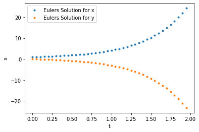
Let \(\frac{d\vec{X}}{dt}=f(\vec{X},t)\), we want to find \(\vec{X}(t)\) over \(t\in[0,2)\), given that \(\vec{X}(t)=[x,y]\), \(\vec{X}(0)=[1,0]\) and \(f(\vec{X},t) = [x-y,y-x]\).
def f(X,t): # the function f(X,t) now takes a vector X as input
    """
    This function returns the value of the function f(X,t) = [X[0]-X[1],X[1]-X[0]].

    Parameters:
    -----------
    X: numpy array
        The value of the vector X.
    t: float
        The value of time t.

    Note: Here the function takes both X and t as input however only X is used in the function. A different time-dependent function can utilize the time variable t.
    """
    x,y = X # the first and the second elements of X are assigned to x and y
    return np.array([x-y,y-x])

epsilon = 0.01 # define timestep

t = np.arange(0,2,epsilon) # define an array for t
X = np.zeros((2,t.shape[0])) # initialize an array for x

X[:,0]= [1,0] # set initial condition

for i in range(1,t.shape[0]):
    X[:,i] = epsilon*f(X[:,i-1],t[i-1])+X[:,i-1] # Euler Integration Step

# Plot the solution
plt.plot(t[::5],X[0,::5],".",label="Euler's Solution for x")
plt.plot(t[::5],X[1,::5],".",label="Euler's Solution for y")
plt.xlabel("t")
plt.ylabel("x")
plt.legend()
plt.show()
A Generalized function for Euler Integration
Here we rewrite the code in a modular fashion and cast the integrator as a function that takes in 3 inputs ie. the function \(\vec{f}(\vec{y},t)\) where \(\frac{d\vec{y}}{dt}=f(\vec{y},t)\), the time array, and initial vector \(\vec{y}_{0}\). We will find this form to be particularly useful when we use TensorFlow functions to code the integrator. Further, it allows us to write multiple integrating functions (for example Euler or RK4) within the same class and call a specific integrator as needed. In addition we also introduce a function to ensure that the correct inputs are given to the integrator failing which an error message is generated.
Algorithm
Get the required inputs: function \(\vec{f}(\vec{y},t)\), initial condition vector \(\vec{y}_0\) and time series \(t\). Entering a time series \(t\) allows for greater control over \(\epsilon\) as it can now vary for each time-step.
Check if the input is of the correct datatype ie. floating point decimal.
Allocate a matrix to hold the output.
At each time step, perform the update \(\vec{y}\) using the Euler method with and store it in the output matrix.
Return the output time series [number of equations \(\times\) iterations] matrix.
def check_type(y,t): # Ensure Input is Correct
    """
    This function checks the type of the input to ensure that it is a floating point number.
    """
    return np.issubdtype(y.dtype,np.floating) and np.issubdtype(t.dtype,np.floating)

class _Integrator():
    """
    A class for integrating a function using the Euler method.
    """

    def integrate(self,func,y0,t):
        """
        This function integrates the function func using the Euler method.

        Parameters:
        -----------
        func: function
            The function to be integrated.
        y0: float
            The initial condition.
        t: numpy array
            The time array.
        """
        time_delta_grid = t[1:] - t[:-1] # define the time step at each point

        y = np.zeros((y0.shape[0],t.shape[0])) # initialize the array for y
        y[:,0] = y0 # set the initial condition

        for i in range(time_delta_grid.shape[0]): # loop through the time steps
            y[:,i+1]= time_delta_grid[i]*func(y[:,i],t[i])+y[:,i] # Euler Integration Step
        return y

def odeint_euler(func,y0,t):
    """
    This function integrates the function func using the Euler method implemented in the _Integrator class.

    Parameters:
    -----------
    func: function
        The function to be integrated.
    y0: float
        The initial condition.
    t: numpy array
        The time array.
    """
    y0 = np.array(y0) # ensure y0 is a numpy array
    t = np.array(t) # ensure t is a numpy array
    if check_type(y0,t):
        return _Integrator().integrate(func,y0,t) # return the integrated function
    else:
        print("Error: Inputs must be floating point numbers.") # print error message
solution = odeint_euler(f,[1.,0.],t) # integrate the function given the initial condition

# Plot the solution
plt.plot(t[::5],solution[0,::5],".",label="Euler's Solution for x")
plt.plot(t[::5],solution[1,::5],".",label="Euler's Solution for y")
plt.xlabel("t")
plt.ylabel("X")
plt.legend()
plt.show()

Runge-Kutta Methods for Numerical Integration
Euler’s method \(x_{n+1}=x_n + \epsilon f(x_n,t_n)\) calculates the solution at \(t_{n+1}=t_n+\epsilon\) given the solution at \(t_n\). In doing so we use the derivative at \(t_{n}\) though its value may change throughout the interval \([t,t+\epsilon]\). This results in an error of the order \(\mathcal{O}(\epsilon^2)\). By calculating the derivatives at intermediate steps, one can reduce the error at each step. Consider the following second order method where the slope is calculated at \(t_{n}\) and \(t_n+\frac{\epsilon}{2}\).
This method is called the second order Runge-Kutta method or the midpoint method.

Above is a schematic description of the second order Runge-Kutta method. The blue curve denotes a solution of some differential equation.
We can reduce errors by calculating additional derivatives. One of the most commonly used integrators is the fourth-order Runge-Kutta Method or RK4 method, that is implemented below:
Note that this numerical method is again easily converted to a vector algorithm by simply replacing \(x_i\) by the vector \(\vec{X_i}\). We will use this method to simulate networks of neurons.
Generalized RK4 Method in Python
We can now modify the Euler Integration code implemented earlier with a generalized function for RK4 that takes three inputs - the function \(f(\vec{y},t)\), where \(\frac{d\vec{y}}{dt}=f(\vec{y},t)\), the time array, and an initial vector \(\vec{y_0}\). The code can be updated as follows,
def check_type(y,t): # Ensure Input is Correct
    """
    This function checks the type of the input to ensure that it is a floating point number.
    """
    return np.issubdtype(y.dtype,np.floating) and np.issubdtype(t.dtype,np.floating)

class _Integrator():
    """
    A class for integrating a function using the Runge-Kutta of order 4 method.
    """
    def integrate(self,func,y0,t):
        """
        This function integrates the function func using the Runge-Kutta of order 4 method.

        Parameters:
        -----------
        func: function
            The function to be integrated.
        y0: float
            The initial condition.
        t: numpy array
            The time array.
        """
        time_delta_grid = t[1:] - t[:-1] # define the time step at each point

        y = np.zeros((y0.shape[0],t.shape[0])) # initialize the array for y
        y[:,0] = y0 # set the initial condition

        for i in range(time_delta_grid.shape[0]): # loop through the time steps
            k1 = func(y[:,i], t[i])# RK4 Integration Steps replace Euler's Updation Steps
            half_step = t[i] + time_delta_grid[i] / 2
            k2 = func(y[:,i] + time_delta_grid[i] * k1 / 2, half_step)
            k3 = func(y[:,i] + time_delta_grid[i] * k2 / 2, half_step)
            k4 = func(y[:,i] + time_delta_grid[i] * k3, t + time_delta_grid[i])
            y[:,i+1]= (k1 + 2 * k2 + 2 * k3 + k4) * (time_delta_grid[i] / 6) + y[:,i]
        return y

def odeint_rk4(func,y0,t):
    """
    This function integrates the function func using the Runge-Kutta of order 4 method implemented in the _Integrator class.

    Parameters:
    -----------
    func: function
        The function to be integrated.
    y0: float
        The initial condition.
    t: numpy array
        The time array.
    """
    y0 = np.array(y0) # ensure y0 is a numpy array
    t = np.array(t) # ensure t is a numpy array
    if check_type(y0,t):
        return _Integrator().integrate(func,y0,t) # return the integrated function
    else:
        print("Error: Inputs must be floating point numbers.") # print error message
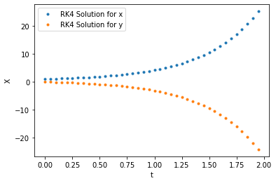
solution = odeint_rk4(f,[1.,0.],t) # integrate the function given the initial condition

# Plot the solution
plt.plot(t[::5],solution[0,::5],".",label="RK4 Solution for x")
plt.plot(t[::5],solution[1,::5],".",label="RK4 Solution for y")
plt.xlabel("t")
plt.ylabel("X")
plt.legend()
plt.show()
Exercise, Solve the differential equations describing the dynamics of a simple pendulum the using Euler and RK4 methods. The equation of motion of a simple pendulum is given by:
where \(L\) = Length of String and \(\theta\) = angle made with vertical. This second order differential equation may be written as two first order coupled equations as follows:
#####################################
# Problem Hint for the Euler Method #
#####################################

# # Note: Uncomment and complete the code below to practice the Euler method.

# epsilon  = ... # define the resolution of the simulation
# t = ... # define the time array

# g = ... # define the value of the acceleration due to gravity
# L = ... # define the value of the length of the pendulum

# def f(X,t): # Create a new function F(X,t) where X is a vector of the form [theta,omega] and t is the time.
#     """
#     This function defines the differential equation for the pendulum.

#     Parameters:
#     -----------
#     X: numpy array
#         The state vector of the pendulum given by [theta,omega].
#     t: float
#         The time.
#     """
#     theta = ... # extract theta from X
#     omega = ... # extract omega from X
#     dtheta = ... # define the derivative of theta
#     domega = ... # define the derivative of omega
#     return np.array([dtheta, domega]) # return the derivative of state vector X

# solution = odeint_euler(...) # Use the Euler method to solve the pendulum problem

# # Plot the solution
# plt.plot(...,".",label="Euler's Solution for theta")
# plt.plot(...,".",label="Euler's Solution for omega")
# plt.xlabel("t")
# plt.ylabel("theta/omega")
# plt.legend()
# plt.show()

# # Now try to implement the Runge-Kutta of order 4 method to solve the pendulum problem by yourself.